| Ch 7. Incompressible and Inviscid Flow | Multimedia Engineering Fluids | ||||||
|
Bernoulli's Equation |
Flow Measurements |
Superposition of Flows |
Flow around Cylinder |
||||
| Superposition of Flows | Case Intro | Theory | Case Solution | Example |
| Chapter |
| 1. Basics |
| 2. Fluid Statics |
| 3. Kinematics |
| 4. Laws (Integral) |
| 5. Laws (Diff.) |
| 6. Modeling/Similitude |
| 7. Inviscid |
| 8. Viscous |
| 9. External Flow |
| 10. Open-Channel |
| Appendix |
| Basic Math |
| Units |
| Basic Fluid Eqs |
| Water/Air Tables |
| Sections |
| eBooks |
| Dynamics |
| Fluids |
| Math |
| Mechanics |
| Statics |
| Thermodynamics |
| ©Kurt Gramoll |
|
|
||
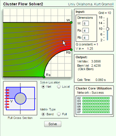 Numerical Solution of Stream Function |
It was shown previously that two-dimensional incompressible, inviscid, and irrotational flow can be described by the velocity potential, φ, or stream function, ψ, using the Laplace's equation: In the following sections, some simple plane potential flows (e.g., uniform flow, source and sink, vortex and doublet) will be introduced. Also, since Laplace's equation is linear, various solutions can be combined to form other solutions. Therefore, some of the real flow problems (e.g., half-body) are obtained by combining these simple plane potential flows using the method of superposition. Normally, the stream function and/or velocity potential equation (Laplace's Equation) is solved easily using finite difference methods or finite element methods. An example of this is given in the graphic. |
|
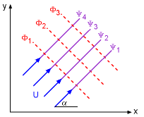
| Uniform Flow |
||
|
|
Uniform flow is the simplest form of potential flow. For flow in a specific direction, the velocity potential is φ = U (x cosα + y sinα) while the stream function is ψ = U (y cosα - x sinα) where α represents the angle between the flow direction and the x-axis (as shown in the figure). Recall that the velocity potential and stream function are related to the component velocity in the 2 dimensional flow field as follows: Cartesian coordinates: Cylindrical coordinates: |
|
|
|
||
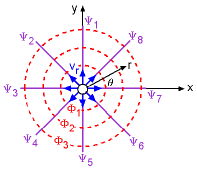
| Source and Sink |
||
|
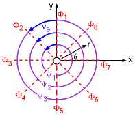
When a fluid flows radially outward from a point source, the velocities are vr = m / (2πr) and vθ = 0 where m is the volume flow rate from the line source per unit length. The velocity potential and stream function can then be represented as respectively. When m is negative, the flow is inward, and it represents a sink. The volume flow rate per unit depth, m, indicates the strength of the source or sink. Note that as r approaches zero, the radial velocity goes to infinity. Hence, the origin represents a singularity. As shown in the figure, the equipotential lines are given by the concentric circles while the streamlines are the radial lines. |
||
| Vortex |
||
|
|
A vortex can be obtained by reversing the velocity potential and stream functions for a point source such that φ = Kθ and ψ = -K ln(r) where K is a constant indicating the strength of the vortex. Now, the equipotential lines are radial lines while the streamlines are given by the concentric circles. The velocities of a vortex are, vr = 0 and vθ = K/r The strength of a vortex can be described using the concept of circulation (Γ), which is defined as, |
|
| Doublet |
||
|
|
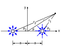
By combining a source and a sink of equal strength using the method of superposition, the stream function is given by ψ = ψsource + ψsink = -(m/2π) (θ1 - θ2) Through considerable manipulation (i.e., geometric relationships and
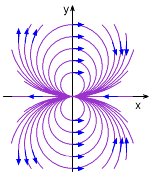
trigonometric identities), the above equation can be rewritten as For small values of a gives, A doublet is obtained by letting the distance between the source and sink approach zero (i.e., distance "a" tends to zero) which means r/(r2 - a2) -> 1/r. The stream function for a doublet then becomes ψ = -Ksinθ/r where K is a constand equal to ma/π, and is called the strength of the doublet. The streamlines of a typical doublet are shown in the figure. The corresponding velocity potential is φ = Kcosθ/r For simplicity, the details of the velocity potential derivation are not given here. Students are encouraged to go through the above derivation process themselves for practice. |
|
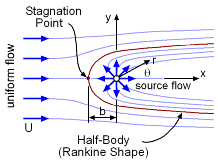
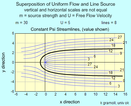
| Flow around a Half-Body |
||
|
|
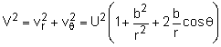
Flow around a half-body (or commonly referred to as a Rankine shape) can be obtained by the superposition of a uniform flow with a source. The combined stream function is given by ψ = ψuniform flow + ψsource = U r sinθ + (m/2π) θ and the corresponding velocity potential is The velocity components are given by Instead of using the source strength, m, it is common to describe the velocities in terms of b (distance from the source to the stagnation point). The b distance is helpful in graphing and describing the half-body or Rankine shape. The b term can be related to m by considering the stream line going through the stagnation point (θ = π and r = b) where vr and vθ are zero. For vr , this gives, 0 = U cosπ + m / (2πb) b = m / (2πU) |
|
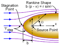 Flow Past a Half-Body (Rankine Shape) |
Using b in place of m, the total velocity at any point in the flow field is, Now back to the interesting half-body or Rankine shape. The stream line that goes through the stagnation point (θ = π and r = b) is also the stream line that defines the surface edge, ψstag =
U b sinπ + (m/2π) π By replacing this streamline with a solid boundary, one can then clearly see that flow around a half-body can indeed be represented by the superposition of a uniform flow with a source. The equation describing the stream function , ψstag, going through the stagnation point can be determined by, m/2 =
U r sinθ + (m/2π) θ Or in terms of b, b (π - θ) = r sinθ This equation gives the surface equation in polar coordinates, r and θ. |
|
|
||

Practice Homework and Test problems now available in the 'Eng Fluids' mobile app
Includes over 250 free problems with complete detailed solutions.
Available at the Google Play Store and Apple App Store.