MATHEMATICS - THEORY
|
| |
|
Curve Sketching
|
| |
|
The concepts of domain, limits,
derivative, extreme values, monotonicity and concavity have been introduced.
Now it is time to combine these concepts together to plot functions
and reveal key features of the functions. In order to draw a function,
many issues need to be considered. They are domain, intercepts, symmetry,
asymptotes, monotonocity, extreme value, concavity and inflection points.
Each one is discussed below. |
| |
|
|
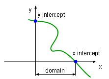
Domain and Intercepts |
|
- Domain
Domain is the range on which
the function is defined. Estiblishing or setting the domain is the first
step of plotting.
- Intercepts
The intercepts refer to the intersection of the curve and y axis or x axis. In
another words, intercepts are the points where the graph cross the axis. By
setting x equals 0, the intersection of the curve and the y axis can be found.
Theoretically, letting y equals 0, the intersection of the curve and the x
axis can be calculated. However, in engineering, complicated functions such
as high order polynomial functions might have multiple x intercepts that can
make the calculation process difficult. In this case the value of x can be
estimated.
- Symmetry
Symmetry can aid in plotting. For some cases only half the curve is determined
and reflected about the symmetry axis or point. Although a curve can have symmetry
with respect to a line or a point, only symmetry with respect to origin, y
axis and periodic symmetry will be introduced here.
|
| |
|
|
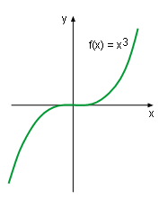
Function f(x) = x3 |
|
- Symmetry about origin
If f(-x) = -f(x) in the domain of the function, then it is an
odd function. The curve of an odd function is symmetry about the origin.
This concept can be better understand by finding the symmetry of function f(x) = x3.
First substitute -x into function f(x) = x3 to
check the odevity of the function. That gives
f(-x) = (-x)3 = -x3 = -f(x)
Since f(-x) = -f(x) , function f(x) = x3 is an odd function,
and thus it is symmetry about the origin. This conclusion is confirmed by
its graphic on the left.
|
| |
|
|
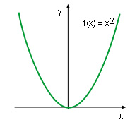
Function f(x) = x2 |
|
- Symmetry about y axis
If f(-x) = f(x) in the domain of the function, then the function is an even
function. The curve of an even function is symmetry about the y axis.
This concept can
be better understand by finding the symmetry of function f(x) = x2.
First substitute -x into function f(x) = x2 to
check the odevity of the function. That gives
f(-x) = (-x)2 = x2 = f(x)
Since f(-x) = -f(x), function f(x) = x2 is an even function
and is symmetry about the y axis. This conclusion is confirmed by
its graphic on the left.
|
| |
|
|
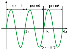
Function f(x) = sinx |
|
- Periodic symmetry
If f(x) = f(x + b) where b is a positive constant in the domain of the function,
then the function is an periodic function and the smallest b is the period
for this function. The curve of a period function repeats every period.
For example, function f(x) = sinx is a periodic function with a period of 2π. The
entire diagram of the sinx can be plotted by translating the graph of the curve
in the range of 0 and 2π as shown
on the left.
|
| |
|
|
| |
|
- Asymptotes
Basically there are three kinds of asymptotes including horizontal asymptotes,
vertical asymptotes, and slant asymptotes. Each one of these will be
discussed in the following paragraphs.
|
| |
|
|
 Horizontal asymptotes I
Horizontal asymptotes II |
|
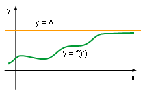
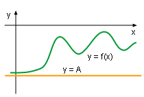
- Horizontal asymptotes
The line y = A is called a horizontal asymptote of the curve y = f(x)
if
 or or 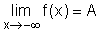
Although the curve of the function approaches the line y = A, it
never actually reaches or crosses.
|
| |
|
|
Vertical asymptotes I
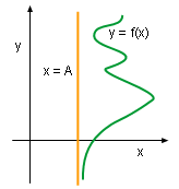
Vertical asymptotes II
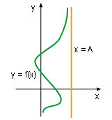
Vertical asymptotes III |
|
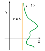
- Vertical asymptotes
The line x = A is called a vertical asymptote of the curve y = f(x)
if any of the following statements is true:
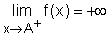
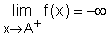
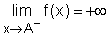
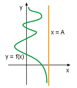
Vertical asymptotes IV
|
| |
|
|
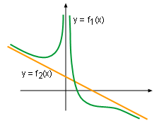
Slant asymptotes
|
|
- Slant asymptotes
In the case where the curve approaches a line that is neither horizontal
nor vertical, such as the function shown on the left, that line is called
an oblique
or slant asymptote of the curve. In other words, if
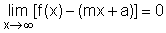
then the line y = mx + a is called a slant asymptote.
|
| |
|
|
| |
|
- Monotonocity
Using the test for monotonicity functions to find the increasing and
decreasing interval of the function. If the derivative is larger than zero for
all x in (a, b), then the function is increasing on [a, b]. If the
derivative is less than zero for all x in (a, b), then the function
is decreasing
on [a, b].
|
| |
|
|
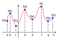
Local
extreme value |
|
-
Local extreme value
In engineering and economics, many problems are related to local maximum
and minimum values, such as finding the biggest volume and lowest
price. Local extreme values are key features
of these types of curves. In order to find the local extreme value of
a function, the critical point need to be calculated first.
Although many methods can be used
to separate the local maximum values from the local minimum values, the first
derivative test and the second derivative
test are the most commonly used methods and are listed below.
|
| |
|
|
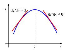
Local Maximum |
|
-
First derivative test
If the value of the function's derivative changes from positive to negative
at x = c, then the function has a local maximum at this point.
On the other hand, if the value of the function's derivative changes
from negative to positive at x = c,
then the function has a local minimum at this point.
-
Second derivative test
If at a point the first derivative of the function is 0 and second derivative
is larger than 0, then the function has a local minimum at this point. On the
other hand, if at a point, the first derivative of the function is 0 and the
second derivative is less than 0, then the function has a local maximum at
this point.
|
| |
|
|
| |
|
-
Concavity and inflection points
When a curve is increasing, the bend upward and bend downward curve gives
different tendency of a curve. It is similar for a decreasing curve.
Computing the second derivative of the function and using the test
for concavity
can figure out the
the bend
direction. When the second derivative is larger than 0, the curve is
concave downward. On the other hand, when the second derivative is
less than 0, the curve is concave upward.
|
| |
|
|
| |
|
- Sketching
With the above information, a rough graph can be plotted. First draw
the x, y axis and the asymptotes. Second plot the intercepts, extreme
values, and the inflection points. Finally, draw the curve passing
all these points, increase and decrease according the the test
for monotonicity functions, and bend the curve according to the function's
concavity.
|
| |
|
|